Chatting with Qbo

You can ask Qbo questions using natural language. This gives you a different search experience with a simpler, conversational tone. For example, you can enter, What was my top selling product last quarter?, instead of typing something like top product by sales in the last quarter. You can also speak your query using the voice-to-text capability of your operating system.

Ask your administrator to enable voice. Click on the icon in the conversation pane and start talking.

Query space

A query space in a thread allows you to ask queries using more natural, speech-like search language. Qbo ignores extraneous words like What are the or Can you show me.

To speak the query using the voice-to-text capability of your operating system, ensure that your microphone is enabled, connected, and working correctly. Click on the microphone to begin voice input, which is translated to text in the search bar.

The query search only supports queries in English language.

Autocompletions

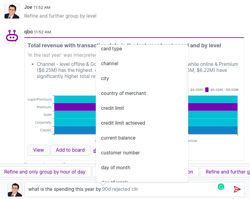
The autocomplete feature in the Qbo queryBot provides a list of suggestions to select from as you type your query. It suggests words based on the tables that exist in your data.

NLP Diagnostics

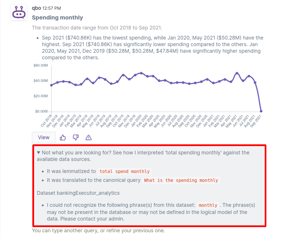
NLP diagnostics shows the interpretation of the input phrase and how it has been understood and processed. The NLP diagnostics may contain the transformed utterance after spell checking, lemmatization, thesaurus normalization, and unrecognized phrases.

NLP diagnostics appear underneath every query if the diagnostics feature is enabled for that user.

To disable the diagnostics feature, you must either have Qbo administrator access or contact your administrator.

If you have admin access:

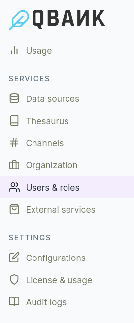
Go to the admin section and click Users & roles.
Click the ROLES and PERMISSIONS tab and click the Create new roles button.
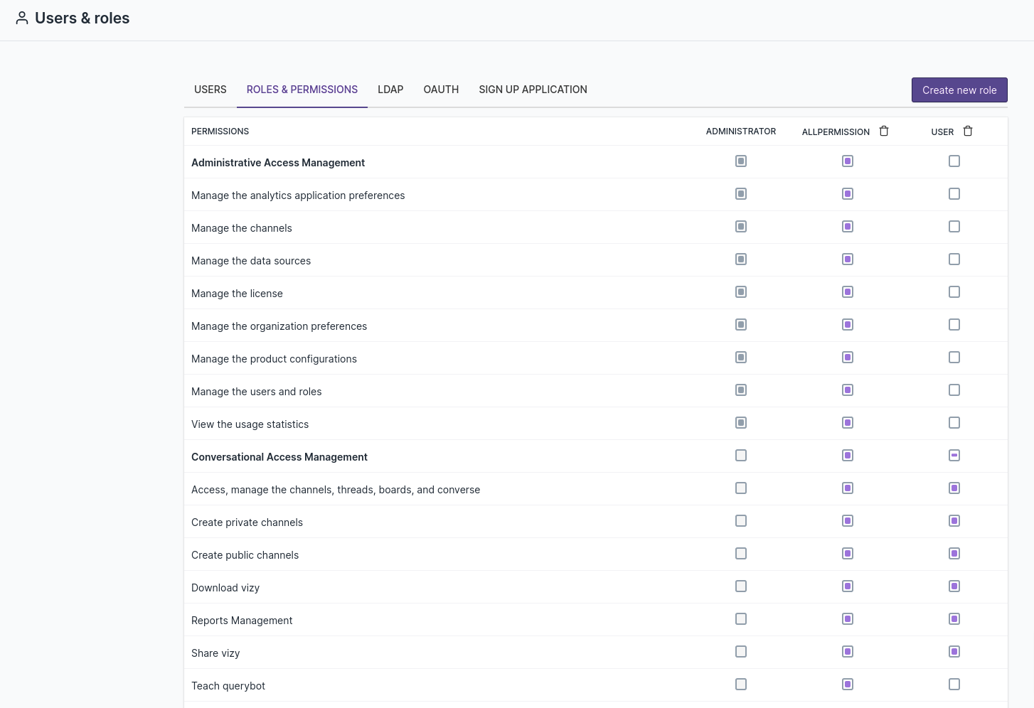
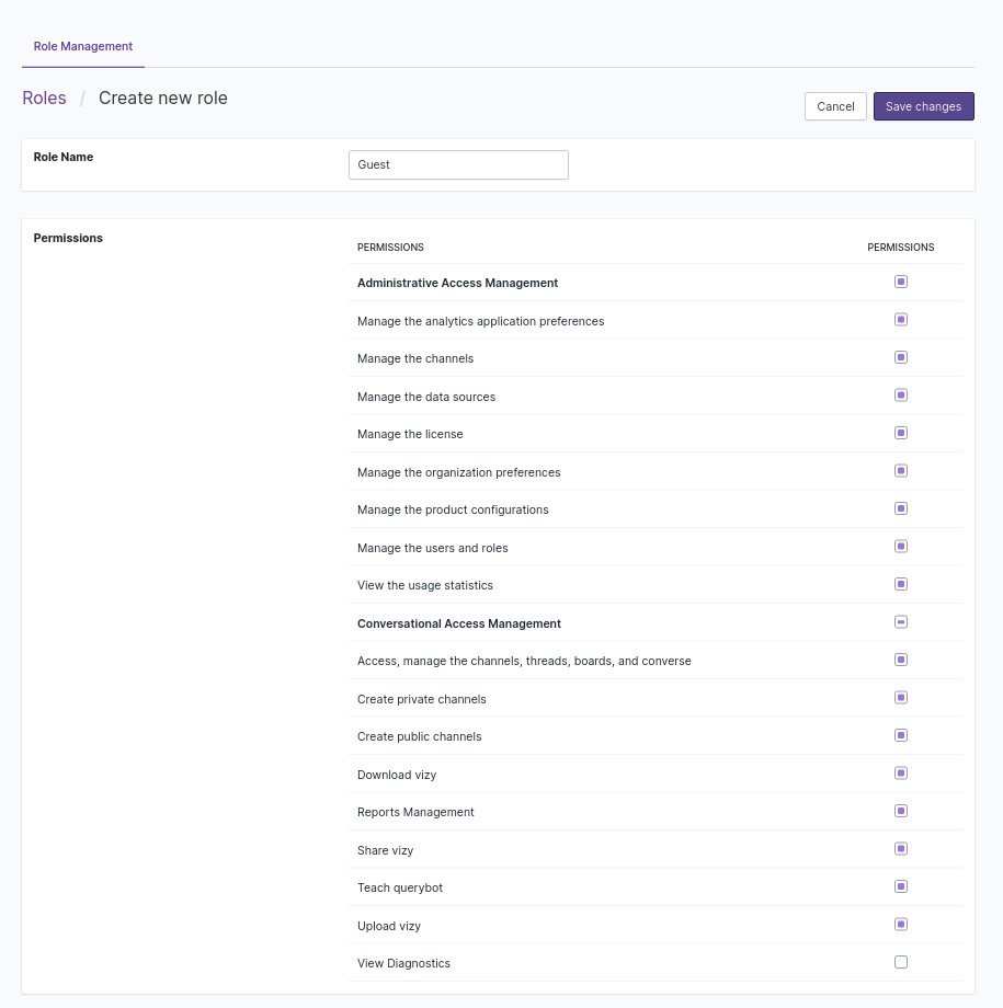
Create a new role, select all the roles and permissions, unselect View Diagnostics, and click Save changes.
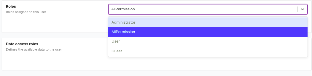
To apply a new role to a user, go to a USERS tab, select the user whose role you want to change. In the Roles section, select the new role you created and click the Save button.

Qbo will disable the diagnostics feature for that user.

Types of queries

There are several types of autogenerated queries such as Single Object Profile Queries, Selection Queries, Aggregation Queries, Trend Queries, Comparison Queries, and Variance Queries.

Single object profile queries

Ask about the attributes of a single entity object. This object can be identified by a unique key. For example:

What is the age and date of birth of customer John Smith

In this example, we assume that “John Smith” is a value of an attribute like name that is the primary key of the customer entity.

Selection queries

Selection queries are queries on a single entity that list out all values (or instances) of the entity that satisfy certain properties. The base form of a selection query is:

What are the <Entities>?

This lists out all the instances of a certain entity (usually all the rows in a certain table that corresponds to that entity).

For example, What are the transactions lists out all the transaction instances found in the DB. More specifically, it generates a list (or table) of different entity instances and this includes those attributes of the entity that are marked as displayed = true.

There are several clauses that you can use to give more specifics of exactly which entities you want.

With filters:

Filter based on one attribute.

For example, What are the dates and values of the transactions with amount greater than 40?

String attribute filters, including equal, starting with, ending with, not starting with, not ending with, containing, not containing.

Numeric attribute filters, including equal, greater than, lesser than, greater than or equal, lesser than or equal, between 2 numbers.

Date attribute filters, including:

after < date >

before < date >

on or after < date >

on or before < date >

on a < Day of Week >, e.g. on a Sunday

in < Month >of any year, e.g. in January of any year

in < Month > < Year >, e.g. in January 2019

between < data > and < date >

(this | in the last) (week | month | quarter | year)

Boolean attribute filters - checking for true or false:

What are the transactions that are not cancelled.

What are the transactions that are cancelled.

Existential filters - not NULL:

What are the customers without a card.

Filter based on multiple attributes:
- Where multiple filters can be combined with “and” and “or”.
Filter based on attribute in referenced table:
- What are the transactions from customers in countries with population at least 50000000.
Filter based on aggregated attribute:
- What are the customers with total count of transactions greater than 100.

Note

The aggregated attribute might be part of the same entity or in a referenced entity.

Top k

Top k (or bottom k) entities by their total count (or bottom k):
- What are the top 5 products.
This implicitly orders the products by their total count.
Top k (or bottom k) entities ordered by an attribute:
- What are the top 5 products in order of price.
- What are the names and prices of the top 5 products in order of price
Top k (or bottom k) entities ordered by an aggregated attribute (usually from a referenced entity):
- What are the top 5 customers in order of their total purchase amount.

Refinements for selection queries:

There are several kinds of refinements possible.

Lets start with a first query: What are the last 5 transactions with quantity less than 3 and with amount at least 10.5?

Here are various possible refinements:

Refine and show the first 10 (this is equivalent to):

What are the first 10 transactions with quantity less than 3 and with amount at least 10.5?
Refine and show the first 10 in order of the time (this is equivalent to):

What are the first 10 transactions in order of the time with quantity less than 3 and with amount at least 10.5?
Refine and only show those with quantity less than 3 (this is equivalent to):

What are the first 10 transactions in order of the time with quantity less than 3?
Refine and restrict to show those with amount at least 10.5 (this is equivalent to):

What are the first 10 transactions in order of the time with quantity less than 3 and with amount at least 10.5?
Refine and expand to show those with quantity greater than 6 (this is equivalent to):

What are the first 10 transactions in order of the time (with quantity less than 3 and with amount at least 10.5) or with quantity greater than 6?
Refine and only show those from customers in countries with population at least 50,000,000 (this is equivalent to):

What are the first 10 transactions in order of the time from customers in countries with population at least 50000000?
Refine and also show the ids (this is equivalent to):

What are the ids and other details of the first 10 transactions in order of the time from customers in countries with population at least 50000000?
Refine and only show the quantities and amounts (this is equivalent to):

What are the quantities and amounts of the first 10 transactions in order of the time from customers in countries with population at least 50000000?
Refine and only show the unique quantities and amounts (this is equivalent to):

What are the unique quantities and amounts of the first 10 transactions in order of the time from customers in countries with population at least 50000000?

Aggregation queries

Aggregation queries are queries on a single entity that calculate one or more metrics for the entity.

The base form of an aggregation query is:

What is the <Aggregation Function> <Attribute> of the <Entities>?

This calculates an aggregation on an attribute for all instances of an entity.

For example, What is the total amount of the transactions calculates a sum of the amounts for all transactions.

Depending on the type of attribute, there are several aggregation functions that can be applied:

For numeric or datetime related attributes, we can calculate maximum and minimum.
For numeric attributes, we can calculate average and total.
For datetime attributes, we can calculate earliest and latest.
For all attributes, we can calculate number of unique values.

It is also useful to think of aggregation queries in terms of metrics and dimensions. A metric is a quantitative measurements, usually as a result of applying an aggregation function on an attribute of an entity. A dimension is an attribute of the entity that can be used for filtering, grouping or ordering the metric calculation.

There are several clauses that you can use to further tailor the aggregations produced:

Aggregate after filtering based on one attribute. This filter can be based on any attribute of the entity, including date, numeric and string attributes.

For example, What is the total number of the transactions that occurred in the last month?

This first filters all the transactions based on a certain attribute, and then calculates an aggregate on the resulting dataset. Note that in this particular example, the phrase occurred in has been associated with the transaction date attribute in transactions.

It can be extended to filtering on multiple attributes.
Group By Clause.

For example, What is the total amount of the transactions by product code

This first groups all transactions by product code and then calculates the total amount for each product code. There are different grouping logics based on the data type of attribute used for grouping:
- If it’s a string data type, then the unique values of the strings become the groups.
- If its an integer data type:
  - Unique values of the integers can become groups.
  - We can further bucket the integer values into 4 (quartiles), 10 (deciles) or a user specified number of buckets.
- If its a float data type, since it’s difficult to group by unique float values, Qbo only supports bucketing the floats into ranges, into 4 (quartiles), 10 (deciles) or a user specified number of buckets.
- If it’s a date data type:
  - Unique values of the integers can become groups.
  - We can further bucket the dates by day, week, month, quarter or year. This effectively gives us trend queries.
Multiple Group By Clauses.

For example, What is the total amount of the transactions by product code and by amount quartiles

This first groups all transactions by product code and then calculates the total amount for each product code.
Group By and Having Clause. A “having” clause essentially allows filtering the results of a group by query based on the value of some aggregate on each group.

For example, What is the total amount of the transactions by product code having total amount greater than 250.0. This first does an aggregation to calculate the total amount of all transactions for each product code, and then returns those values of the product code where this total amount is greater than 250.0.

The key difference between an “attribute filter” clause and a “having” clause is that attribute filters are filters applied on attributes (or dimensions) of entities, while having clauses are filters applied on metrics.
Top k. In the context of aggregation queries, a top k query finds the top k among groups.

For example:
- What are the 3 most common quantities of the transactions: This orders the quantities by their total count. It first groups the transactions by quantity and orders the groups by the total count.
- What are the top 3 product codes of the transactions in order of the maximum amount: First groups the transactions by product code and orders the groups by the max amount.
- What are the top 3 months based on delivery dates of the transactions.
Top k and Having Clause.

For example, What are the top 3 product codes of the transactions having total number less than 3: This first does an implicit grouping of all transactions by the product code, filters the product codes based on the total number, and then orders the remaining product codes based on the total number.
Top k, Order By and Having Clause.

For example, What are the top 3 product codes of the transactions having total number less than 3 in order of the total amount: This first does an implicit grouping of all transactions by the product code, filters them based on the total number, and then orders them based on the total amount.

We can combine many of the above clauses to create more complex queries such as:

Aggregate and group by, after filtering based on one or more attributes.

Aggregate and group by and show groups having some properties, after first filtering based on one or more attributes.

Refinements to Aggregation Queries

Several kinds of refinements can be applied to aggregation queries.

Lets assume we start with a query like:

What is the total number of the customers by country

Then some possible refinements are:

Refine and group by < attribute >.

For example, Refine and only group by last name: This essentially results removes all previous group bys and now groups by the last name
Refine and further group by < attribute >

For example, Refine and further group by ID quartiles: This adds an additional group by to any previous ones. So, effectively, this query is now equivalent to What is the total number of the customers by last name and by ID quartiles

If we now query: Refine and only group by ID values divided into 5 bins
Refine and only show the < aggregation function > < attribute >.

For example, Refine and only show the maximum ID: This replaces the metric(s) being displayed with the new one computed as < aggregation function > < attribute >.
Refine and also show the < aggregation function > < attribute >.

For example, Refine and also show the total number.

This adds an additional metric to the results.
Refine and only show groups having < aggregation function > < attribute > < comparison phrase >.

For example, Refine and only show groups having total number greater than 10.

The < aggregation function > < attribute > < comparison phrase > essentially acts as a group-level filter. This takes groups that may come from previous group by expressions and only shows those that satisfy the given condition on a metric.
Refine and restrict to show groups having < aggregation function > < attribute > < comparison phrase>.

For example, Refine and restrict to show groups having minimum id exactly 5.

This takes groups that may come from previous group by expressions and filters on the groups and adds an extra filter condition _static. so now it only shows those that satisfy the given condition and any previous conditions
Refine and expand to show groups having < aggregation function > < attribute > < comparison phrase>

For example, Refine and expand to show groups having minimum id exactly 10.

This takes groups that may come from previous group by expressions and filters on them and adds an additional optional condition. Now it only shows those that satisfy the given condition or any previous conditions.
Refine and aggregate those with < attribute-level filter >.

For example, Refine and aggregate those with first name containing “a”.

This filters the dataset used for aggregation. It only calculates the metric on values of the dataset that satisfy the filter conditions.
Refine and restrict to those with < attribute-level filter >.

For example, Refine and restrict to those with first name containing “b”.

This adds an “and” condition to the filters on the dataset used for aggregation. It only calculates the metric on values of the dataset that satisfy this and any previous filter conditions.
Refine and expand to those with < attribute-level filter >.

For example, Refine and expand to those with first name containing “c”.

This adds an “or” condition to the filters on the dataset used for aggregation. It only calculates the metric on values of the dataset that satisfy this or any previous conditions.

More refinements are possible with top-k queries that involve aggregations.

For example, if you start with, What are the top 3 quantities of the transactions?

This orders the quantities based on the total count of each quantity.

Some possible refinements are:

Refine and show in order of the < aggregation function > < aggregated attribute >.

For example, Refine and show in order of the total amount is equivalent to What are the top 3 quantities of the transactions in order of the total amount?

This can also be done with named aggregates.
Refine and show those having < aggregation function > < attribute > < comparison phrase >.

For example, Refine and show those having total number less than 3.
Refine and show values for < attributes >.

For example, Refine and show values for delivery dates is equivalent to What are the top 3 delivery dates of the transactions having total number less than 3 in order of the total amount?
Refine and show the bottom k is equivalent to What are the bottom 5 delivery dates of the transactions having total number less than 3 in order of the total amount?

Let’s take a possible path of refinement queries as an example to see how it is possible to “converse” with your data:

What is the total number of the customers by country?

Refine and only group by last name is equivalent to *What is the total number of the customers by last name?
Refine and further group by id quartiles is equivalent to What is the total number of the customers by last name and by id quartiles?
Refine and only group by id values divided into 5 bins is equivalent to What is the total number of the customers by id values divided into 5 bins?
Refine and only group by country goes back to the original query and is equivalent to What is the total number of customers by country?
Refine and further group by country is equivalent to What is the total number of the customers by country?
Refine and further group by last name is equivalent to What is the total number of the customers by country and by last name?
Refine and only show the maximum ID is equivalent to What is the maximum id of the customers by country and by last name?
Refine and also show the total number is equivalent to What is the maximum id and total number of the customers by country and by last name?
Refine and only show the number of unique first name values is equivalent to What is the number of unique first name values of the customers by country and by last name?
Refine and only show the total number is equivalent to What is the total number of the customers by country and by last name?
Refine and only show the total count goes back to the last group by refinement and is equivalent to What is the total count of the customers by country and by last name?
Refine and only show the maximum ID and minimum ID is equivalent to What is the maximum id and minimum id of the customers by country and by last name?
Refine and also show the total number and number of unique first name values is equivalent to What is the maximum ID and minimum ID and total number and number of unique first name values of customers by country and by last name?
Refine and only show the total number goes back to the last group by refinement and is equivalent to What is the total number of customers by country and by last name?
Refine and only group by country goes back to the original and is equivalent to What is the total number of customers by country?
Refine and show groups having total number greater than 10 is equivalent to What is the total number of customers by country having total number greater than 10?
Refine and show groups having total number less than 2 is equivalent to What is the total number of customers by country having total number greater than 10 or total number less than 2?
Refine and show groups having minimum ID exactly 5 is equivalent to What is the total number of customers by country having (total number greater than 10 or total number less than 2) and minimum ID exactly 5?
Refine and only show groups having total count greater than 10 is equivalent to What is the total count of customers by country having total number greater than 10?
Refine and only show groups having total number greater than 10 goes back to the last group filter refinement and is equivalent to What is the total number of the customers by country having total count greater than 10?
Refine and aggregate those with first name containing “a” is equivalent to What is the total number of customers with first name containing “a” by country having total number greater than 10?
Refine and restrict to those with first name containing “b” is equivalent to What is the total number of customers with first name containing “a” and with first name containing “b” by country having total number greater than 10?
Refine and expand to those with first name containing “c” is equivalent to What is the total number of the customers with first name containing “a” and with first name containing “b” or with first name containing “c” by country having total number greater than 10?

Trend queries

Trend queries are a special type of aggregation query. They involve computing one or more metrics for every time period. This is achieved by grouping the data by day, week, month, quarter or year and then computing the aggregated metrics for each time period.

The base form of a trend query is:

What is the <Aggregation Function> <Attribute> of the <Entities> by <Date Attribute> <Periodicity Unit>?

Where Periodicity Unit is daily, weekly, monthly, quarterly or yearly.

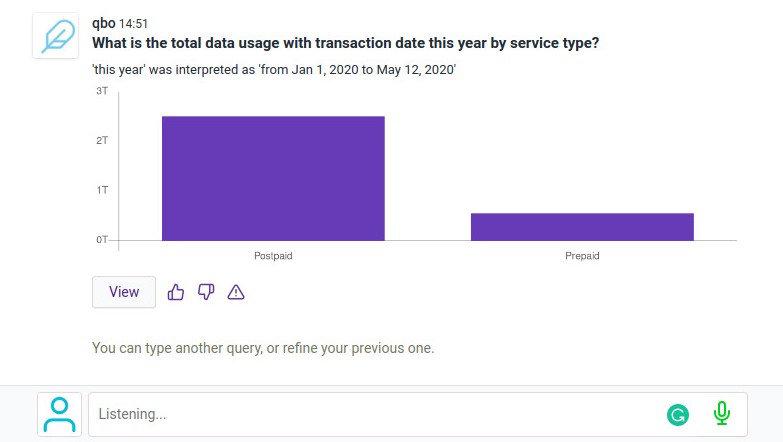
For example, What is the total amount of the transactions by transaction date daily calculates the trend of the total amount of the transactions for each day, based on the transaction date.

Refinements of Trend Queries

Several kinds of refinements to aggregation queries can be applied to trend queries as well.

For example, start with a query like:

What is the total number of transactions by delivery date monthly

Some possible refinements are:

Refine and further group by time weekly: Results in the monthly trend of transaction count being further grouped by week based on the time attribute.
Refine and further group by canceled: Results in a further grouping of the monthly trend by the boolean attribute canceled. It results in two trends, based on whether the transaction was canceled or not.

Comparison queries

Comparison queries allow comparing one or more metrics between two different dates or date ranges. Specifically, Qbo allows comparing a metric for one time period against the previous time period, using these phrases: week-over-week, month-over-month, quarter-over-quarter, and year-over-year.

The base form of a comparison query is:

What is the <Aggregation Function> <Attribute> of the <Entities> <PeriodOverPeriodClause>

Some examples:

What is the total amount of the transactions month-over-month
What is the total amount and average quantity of the transactions month-over-month

Variance queries

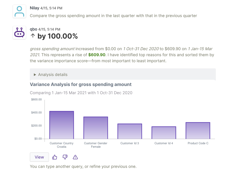
Variance queries allow comparing the values of a metric (also called behavioral aspect) between the two different values of a dimension (also called a related aspect), and analyzing the key reasons for the differences. Qbo digs into different dimensions (or aspects) that are related to the metric to identify the most significant values that explain the difference between the two values of the metric. Qbo ranks the values of each dimension based on the absolute change, percentage change, and significance of the change in comparison to other values in that dimension. It presents the top k values along with additional information about other related metrics.

There are two common types of variance queries:

Comparison based on a time attribute.

Comparison based on a non-time attribute.

Comparison based on a time attribute

This is the most common kind of variance query, and is commonly used to analyze why some metric has increased or decreased in a given time period compared to some baseline. There are two different ways of defining the baseline:

Comparison of the value of a metric between two different periods of time. It is possible for the two different periods to be of different lengths of time – in this case, Qbo just warns about this and proceeds with the analysis. For example:
- Compare the spent amount in the last 3 days with the previous 3 days
- Compare the spent amount in the current week with the previous 3 days
- Compare the spent amount in the last 3 weeks including this week with the previous 3 weeks
- Compare the spent amount in the last 2 months including this month with the previous 3 weeks
- Compare the spent amount in the current week with that in between 2016-08-01 and 2016-08-02
Comparison of the value of a metric on a given time period with an average. The average is computed on the full dataset, and it can be a daily, weekly, monthly, quarterly or yearly average depending on how the time period is defined. For example:
- Compare the spent amount on 2016-07-18 with the average: Compare the spent amount on a given day with the daily average over the whole dataset. The phrase the average is interpreted as daily average by default.
- Compare the spent amount in the last 2 quarters including this quarter with the weekly average: Compare the weekly average of the spent amount in the last 2 quarters including the current quarter so far, with the weekly average over the whole dataset. Averaging period specified for the planned period is used for both time periods.

Comparison based on a non-time attribute

This allows us to compare the value of metric between different products, customers, regions or other non-time dimensions, and analyze the key factors behind the difference. For example:

Compare the spent amount of customer Maryjane Doyle with that of customer Tianna Stanley

Compare the spent amount of customer “Maryjane Doyle” with that of customer Tianna Stanley

Both kinds of variance queries can be further extended with filters such as a time based variance query can be further filtered based upon non-time dimensions. This allows drilling down into differences in the value of the metric along specific dimensions.

For example, we can ask:

Compare the spent amount today with the average yesterday for customer equal to Payton James

Compare the spent amount today with the average yesterday for customer equal to Payton James or customer ends with “Glenn”

Compare the spent amount of customer Maryjane Doyle with that of customer Tianna Stanley for category equals Travel

Note that in the autogenerated phrasing, the filters (like customer equal to Payton James) comes at the very end. Also, note that we don’t as yet support time-based filters.

Refinements

There are several kinds of refinements we can ask on a variance query:

Refine further and show by <aspect>

The base variance query examines values of all relevant related aspects (or dimensions) and ranks them based on their contribution and significance to the overall variance. When we refine by a certain aspect (or dimension), it ranks and displays the values for the specified aspect only.
Refine further and show comparison side-by-side

The default chart for a certain aspect only shows the absolute or percentage difference of the value of the metric between the two periods under consideration. The comparison side-by-side shows information for the two values of the metric for the two time periods (or other dimension values)
Refine further and show top 10 <aspect> with <increase or decrease>

By default the values in an aspect are ranked by a variance significance score that considers a combination of the absolute difference and the relative variance compared to other values in the aspect. However, this refinement allows ranking the aspects just by absolute increase or decrease
Refine further and show for <aspect> <aspect filter>

This refinement allows adding aspect based filters into the analysis, and thus drilling into certain values

For example:

Refine further and show for category equal to Electronic Sales or merchant starts with “APL-”

Variance Importance Score

Values are sorted according to not absolute variance but variance importance score. A score is calculated by multiplying

variance * z-score of variance

where,

z-score = variance - mean of variance for aspect / standard deviation of variance

For example, if we are looking at credit card transaction data, an aspect like merchant might have many unique values, while province might have fewer. When grouped, each province would contribute a large amount to overall variance, because it has many more transactions. However, a merchant might have a significant contribution to variance relative to the number of transactions associated with it. In that case, we would like to be able to present this information to the user. We calculate the score to normalize contribution to variance between aspects with different number of values and pick values that have significant contribution.

NLP queries

So far we have been using only queries that were suggested by the bot through autocompletions. Now, let’s see free-form natural language processing based queries in Qbo. This allows you to type queries as you choose, and the bot will do its best to interpret the utterance in the context of the data in the database. This uses novel NLP algorithms to translate arbitrary natural language text to the relevant queries to the DB.

Some of the key features of Qbo’s NLP are :

Requires no “training” for an initial deployment.

Only requires synonym definitions and phrasing of entities, aggregates and attributes. NLP configuration is done by the administration for the data.

Can get similar queries to ask questions like “did you mean X or Y”.

Qbo uses the ability of the NLP model to understand user queries with no prior training, data preparation or human-driven model building.

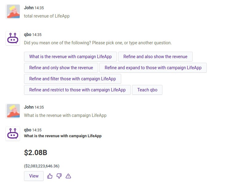
Note

Try an ambiguous question like Total revenue of LifeApp. If your data contains an attribute revenue and an attribute campaign with type lifeApp, then Qbo will request a “Did you mean…” clarification and learn from your response.

Important

Using Cancel Query, you can cancel the clarification loop for converting an NLP query to a canonical one. When the QueryBot tries to match the initial NLP query to a canonical one, it may ask a few questions. That “cancel” stops the process and clears the UI so that you can make a new query.